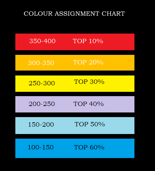
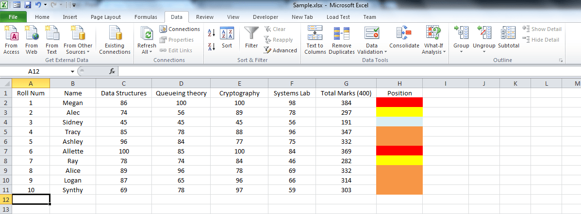
How to sort Microsoft Excel columns by color: – Sorting an Excel document must have never been a tough job. We are all familiar with sorting the excel sheets by a specific or a collection of columns, by using the cell values. But if I tell you that excel sheets can actually be sorted by using colours, would you buy that? Yes or no, that’s exactly what am going to tell you. Excel sheets can indeed be sorted by using colours! You can use the cell values, cell colours, font colours or even cell icons to sort your excel sheets. Here, I have made a sample excel sheet for storing marks of 10 students on different subjects along with their total marks. I have added an extra column named Position. This column actually tells you in what percent of the class the student belongs to. That is, top 10, top 20 and so on. A student with a total mark of 389 would have colour RED assigned on his/her Position column, which means he/she is in the top 10% of the class. Refer to the following chart to see the colour assignment that I have used in my sample excel sheet.
Also read: – How to parse names in Microsoft excel
And here comes the sample excel sheet that I have used. Refer to the colour chart given above, to get a better idea about the sample sheet given below.
At the end of this article, you will actually be able to sort an excel sheet by using only the colour values and not the cell values. Read on, to learn how to hack this simple trick.
STEP 1
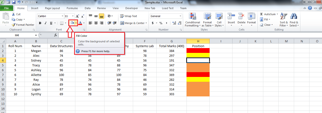
- First of all, let me give you an idea about how to give a cell a specific colour. I know it’s old school basic. But some of us could be new to excel sheets. So, to give a cell a specific colour, click on the cell you want to give the colour to, and then on the fill colour icon, which is located at the top.
STEP 2
- Now from the list of colours, pick the one you want and click on it. Viola, your cell is now coloured! Repeat the same for all the cells.
STEP 3
- Now that you have selected the colours, let’s get to business. Click on the Data tab as shown in the screenshot.
STEP 4
- Highlight the region of your excel sheel that you want sorted. You can drag and select or simply press CTRL+A together.
STEP 5
- Click on the button named Sort. This will open a new window for Sort settings .
STEP 6
- You will have 4 options as shown below. Pick the first one, which is Sort by. From the drop down, choose the column with which you want the sheet to be sorted. Here I have chosen Position, which is the one I have given colours to. Now, as next, from the drop down of Sort of, pick Cell color. Under the drop down of Order, you can see all the colours that you have used to colour your cells. Choose the one which has the highest priority as per your choice. I have chosen Red. Next, pick On Top from the last drop-down menu.
STEP 7
- You can use the Add level button at the top to add a different level. Once you are all done, your Sort window would look somewhat like the given screenshot. You need not specify the last level, as it will be taken care of automatically. Click on OK button when you are all set.
STEP 8
- There you are, your excel sheet is all so sorted and up to go. That’s it.
That’s all it is. You have actually sorted the whole class by using colours only. Yeah, it is cool indeed. Hope you had fun reading and trying out this trick.


