Are you continuously changing the input data range of your Excel spreadsheet as new data becomes available? If yes, then self-updating Excel Charts are enormous time savers. Charts assist you to make decisions based on facts in Excel. They are a pleasant change from staring at data and columns. They also aid in the decision-making process by allowing you to view your results where improvements may be required. The difficulty in handling data and charts is that you constantly have to go back to the chart and update it for new data. Creating Charts in Microsoft Excel may appear daunting, but it is simple to do and you can even make one that updates automatically.
In this article, we will guide you on how to make a chart in Excel spreadsheets that will automatically update when you need to add new data.
Steps involved in creating self-updating charts
We will use an example to show how to create a self-updating excel spreadsheet. For this, I am creating a spreadsheet that will track the number of copies sold in a book shop.
Step 1: Creating an Excel Spreadsheet
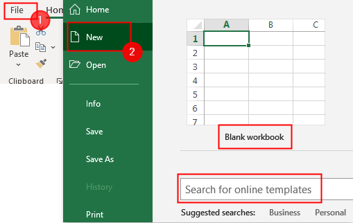
1. Open Excel. Click on File > New > Blank Workbook or Template.

2. Now, start entering your data and create the spreadsheet. The final spreadsheet will look like below.

Step 2: Creating a Table.
Now, you need to format your source data into a table. To do that,
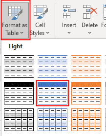
1. Select a cell in the data, Goto Format as table, and click on whichever format you want.

2. A pop-up window appears, leave everything as such, and click OK.


Step 3: Insert the Chart
1. Select the entire table, goto Insert > Recommended Charts.

2. Select the type you want and click on OK.

3. Now, the chart is created and is shown beside your table.

Step 4: Enter the new data
By adding fresh data to the table, we can now see how well our chart functions. Fortunately, this is the most straightforward step of the procedure.
Simply add another column to the right of your existing chart to add new data. Because the formatting of preceding columns is preserved in the Excel table, your date will automatically match what you have entered so far.
Your chart’s X-axis should have already been adjusted to accommodate the new entry. You may now input all of your new data, and the chart will instantly update with the new data.
