In your Excel sheet, you might have a column that you use for calculations, depending on which values of another column could be populated. Though this column need not be visible in the Excel sheet, it cannot be deleted as the values of another column depends on it. In such cases, one great solution would be to hide the entire column. Hiding a column wouldn’t delete the column, but at the same time, it will not be visible anymore.
Also, you might get Excel sheets with hidden columns from someone else. In such cases, you might require to unhide the hidden columns to complete your work efficiently. This article is all about hiding and unhiding columns in an Excel sheet in some simple steps. Read on, to learn how you can easily master this super cool Excel trick.
Section 1: How to Hide Columns in Microsoft Excel
Method 1: By Reducing Column Width to Zero
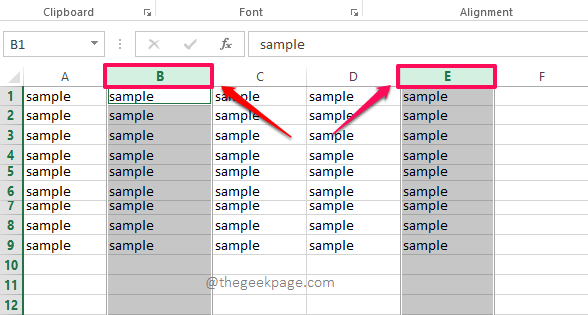
Step 1: Simply select the column that you want to hide by clicking on its header. If you need to hide multiple columns, you need to keep the key CTRL pressed down and then you need to click on the column headers of all the columns that you want to hide.
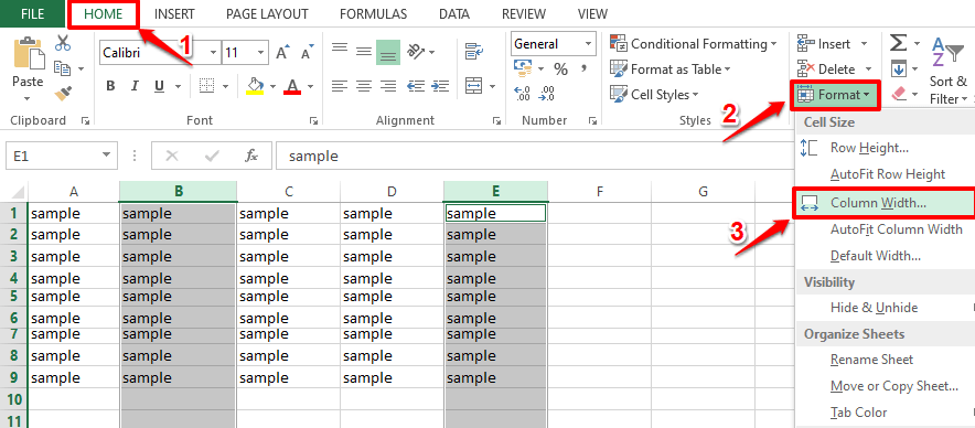
Step 2: Once the columns to hide are selected, click on the HOME tab at the top and then click on the Format dropdown menu under it.
From the list of options available, click on the option named Column Width.
Step 3: In the Column Width window, enter 0(zero) as the width of the column and then hit the OK button.
Step 4: Now if you look at the excel sheet, you can see that the selected columns are hidden. In the example below, columns B and E are hidden.
Method 2: By Choosing Hide Option from the Right-Click Menu of Column Header
This method is very simple. You just need to right click on the column header of the column that you want to hide and then click on the Hide option from the right click context menu.
Note: If you want to hide multiple columns, then press down the CTRL key and click on all the column headers of all the columns that you want to hide, right click on any one of the selected headers, and then click on the Hide option.
Method 3: By Using Hide Option from Format Menu Options
This method is the same as the above method. The only difference is that instead of using the Hide button from the right click context menu, we use it from the Format options.
To hide a column or multiple columns using this method, select the column(s) that you want to hide first.
Click on the HOME tab next, then click on the Format button, click on Hide & Unhide option, and then finally on Hide Columns.
That’s it. This will hide the selected columns.
Section 2: How to Unhide Columns in Microsoft Excel
Method 1: By Dragging and Increasing Column Width
Step 1: If there are hidden columns in your excel, if you look closely, you will be able to the vertical separation of the hidden columns just as shown in the screenshot below. You need to click and drag this vertical separation to unhide the columns that are hidden.
Step 2: Likewise, you can unhide all the hidden columns in your excel. This method works best if you need to unhide only one or two columns.
Method 2: By Choosing Unhide Option from the Right-Click Menu of Column Header
This method also works great if you need to unhide only a couple of columns.
Step 1: If you know a particular column is hidden, you need to select the columns before and after the hidden column. Once you have selected the columns, right click on any one of the selected headers and then click on the Unhide option.
Note: In the example below, column C is hidden. So columns B and D are selected. A right click is made on one of the selected headers, in this example Column D, and then Unhide option is chosen.
Step 2: If you look at the excel, you can see that the hidden column is now unhidden. In the example below, column C was hidden, but now it is visible.
Method 3: By Using Unhide Option from Format Menu Options
Just like in the previous method, select the columns before and after the hidden column(s). Click on the HOME tab next. Then click on the Format dropdown and then on Hide & Unhide option. Finally, click on the option Unhide Columns from the newly expanded context menu.
This will unhide all the columns that are hidden between the selected columns.
Method 4: How to Unhide All Hidden Columns at Once
If there are multiple columns hidden and there are many columns hidden, it will be difficult to unhide them following the methods listed above. In that case, if you wish to unhide all of them at once, then you can follow the method listed in this section.
Firstly, click on the Select All button at the very beginning of your excel cells, which has a diagonal arrow present in it. This will select all the contents in your excel sheet.
As next, click on the HOME tab from the top ribbon. Then click on the dropdown button named Format, then on Hide & Unhide option, and finally on Unhide Columns option.
That’s it. All the hidden columns in your Excel sheet would now be visible to you.
If you have any concerns over any of the steps, please drop us a comment, we are happy to help. Stay tuned!
Note: The same methods can be used to hide or unhide rows as well.


