Having a checklist gets you right on track always. It motivates you to get more things done and thrills you to see things being struck off. Checklists can be created using Excel of course. But not everyone has Excel installed and it would be convenient to get things done through some other reliable way and that’s where Google Sheets comes into the picture from. Anyone with the Internet, a web browser, and a Google account can access Google Sheets and it makes things very convenient.
In this article, we explain in detail how you can easily create a checklist using Google Sheets. More than just creating a checklist, we also explain how you can easily create another column that is dependent on the checklist to populate its values dynamically. Sounds exciting? Well, we promise you it’s more exciting to actually see how this is done. What are you waiting for then? Let’s dive in!
Steps to Create a Checklist in Google Sheets
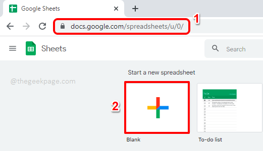
Step 1: The very first step would be to launch Google Sheets. For that, open any browser, preferably Google Chrome, and then click Google Sheets. Once you click on the link, you will have the following window if you’re already logged into your Google account. If you are not logged in, then you will be prompted to log in.
Once you are on the Home page of Google Sheets, click on the Blank tile as shown below to open a blank document.
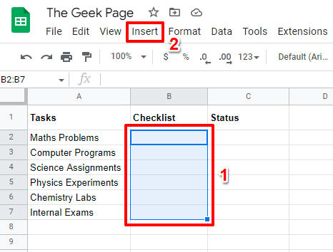
Step 2: Now you can populate the sheet with your data. In the following example, I have 3 columns namely Tasks, Checklist, and Status. Checklist is the column that is going to have the checkboxes. So select the entire Checklist column and then hit the Insert tab at the top ribbon.
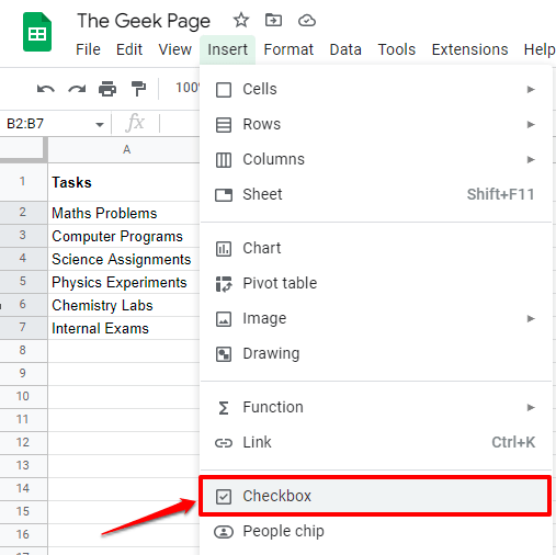
Step 3: Click on the Checkbox option from the list of options that draw out.
Step 4: Now you can see that your Checklist column is readily populated with checkboxes that can be checked and unchecked.
Step 5: You can dynamically check and uncheck the checkboxes by simply clicking on them.
Step 6: Now, let’s populate the Status column dynamically. The logic should be such that if the corresponding checkbox is populated, we should have the Status as TASK DONE and if the checkbox is not populated, then Status should be TASK TO BE DONE.
For that, double click on the first cell of the TASK DONE column and then copy and paste the following formula and then hit the Enter key.
=IF(B2=TRUE, "TASK DONE", "TASK TO BE DONE")
Formula Explanation
Formula checks the first value of the Checklist column and then checks if the checkbox in it is checked or not. Checked means the value is TRUE. If the checkbox is checked, then the function returns Status message as TASK DONE. Else the function returns the message as TASK TO BE DONE.
Note: If the first value of your Checklist column is not in cell B2, then replace B2 with the respective cell id. Also, you can set your own custom messages instead of TASK DONE and TASK TO BE DONE messages.
Step 7: To apply the same formula across the Status column, click on the small square shape present at the bottom right corner of the formula applied cell and then drag it down.
Step 8: Now you can see that the formula is applied across the entire Status column.
Step 9: You can try clicking on any of the checkboxes. In the example below, I have clicked on a checkbox that is not checked. The Status before clicking on the checkbox is TASK TO BE DONE.
Step 10: Once the checkbox is checked, the Status automatically changed to TASK DONE, indicating that our checklist is perfectly working. Enjoy!
Please tell us in the comments section whether you could successfully create a checklist in Google Sheets. If you have any concerns regarding any of the steps, please drop a comment, we are always here to help.
Stay tuned for more amazing tricks, tips, hacks, and how-to articles on your favorite topics.


