To make your Excel documents stand out, it’s always a good idea to splash some colors on them. It’s very easy to select all the cells you want to add colors to, and then choose the colors you prefer. But wouldn’t it be fun if you could color odd rows/columns with one color and even rows/columns with another? Definitely, it will make your Excel documents stand out exceptionally.
So what is the quickest solution using which you can automatically color alternate rows or columns in MS Excel? Well, that’s exactly what we are here today to help you with. Read on, to master this super cool Excel trick with the simplest of the steps possible. Hope you enjoy reading the article.
Section 1: How to Apply Color to Alternate Rows in MS Excel
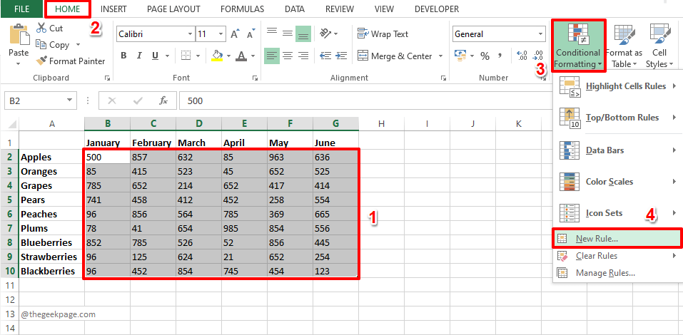
Step 1: Firstly launch the Excel sheet and select the area in your Excel sheet where you want to apply colors to alternate rows.
Then click on the HOME tab from the top ribbon.
As next, click on the Conditional Formatting dropdown button and then click on the New Rule option.
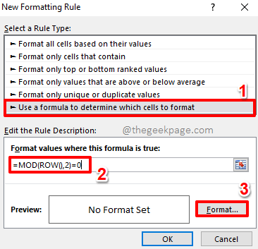
Step 2: On the New Formatting Rule window, under the section Select a Rule Type, click on the last rule type, which is Use a formula to determine which cells to format.
As next, under the section Format values where this formula is true, copy and paste the following formula.
=MOD(ROW(),2)=0
Rule Explanation
The function ROW() would return the row id of the first row in the selected area. The returned value would be 2 as our selected area starts from row number 2. The MOD() function would find the remainder of this row id divided by the number 2, which is equal to 0. If it equates to 0, the formula becomes true and then the formatting that we choose using the Format button would be applied to the row. The same process is repeated for all the rows.
Now let’s decide on the color. For that, click on the Format button.
Step 3: On the Format Cells window, click on the Fill tab at the top of the window.
Now, from the color options available, click on the color that you want to be applied to the even rows in your Excel. You also have other options like Fill Effects, More Colors, Pattern Color, Pattern Style, etc.
Once you are done selecting the color, simply hit the OK button.
Step 4: You will now be back at the New Formatting Rule window. Hit the OK button to proceed.
Step 5: That’s it. You can see that the even rows in your selected area are now formatted with the color of your choice!
If you are ok with having only the even rows being colored and the odd rows being in the default white color, you are all set with alternate row coloring. But if you would like to have the odd rows also to be colored with another color of your choice, then you can go ahead with the steps below. Remember, the steps are all the same, the only difference is in the formula used.
Step 6: Just like before, select the area in which you want the odd rows to be colored.
Once the area is selected, hit the HOME button at the top.
As next, click on the Conditional Formatting button and then choose New Rule.
Step 7: This time also, choose the option Use a formula to determine which cells to format.
Now, copy and paste the following formula on the field Formula values where this formula is true.
=MOD(ROW(),2)=1
Rule Explanation
This time the formula checks whether the row id can be divided by 2 or not. If it can be divided, then the remainder will be 0, else it will be 1. That is, for odd rows the formula, =MOD(ROW(),2)=1, would return true.
Hit the Format button to choose the formatting for the cases where the formula becomes true.
Step 8: You can go to the Fill tab on the Format Cells window and choose a color of your choice.
Hit the OK button to proceed.
Step 9: When you are back at the New Formatting Rule window, hit the OK button to see the alternate coloring in action.
Step 10: That’s it. You now have perfectly shaded alternate rows in your Excel sheet, just like how you wanted it to be. Enjoy!
Section 2: How to Apply Color to Alternate Columns in MS Excel
The steps to alternately color columns are exactly the same as how we would color alternate rows. Obviously, the only difference lies in the rule used, which we will detail in the steps below.
Step 1: Select the range of columns that you want to color alternatively.
Hit the HOME tab from the top ribbon.
Click on the Conditional Formatting dropdown button and then click on the New Rule option.
Step 2: Under the section Select a Rule Type, click on the option Use a formula to determine which cells to format.
Now, under the Format Values where this formula is true, copy and paste the following formula.
=MOD(COLUMN(),2)=0
To set the formatting, click on the Format button.
Step 3: Go to the Fill tab and choose a color of your choice for the even columns.
Hit the OK button.
Step 4: When you are back at the New Formatting Rule window, either hit the Enter key or hit the OK button to proceed.
Step 5: That’s it. You can now see that the alternate even columns are colored using the color you chose.
If you are ok with the odd columns being in the default white color, you can stop right here. But if you would like the odd columns also to be in a specific color that you choose, then you can continue with the steps below.
Step 6: As always, select the area first and then hit the HOME tab from the top ribbon.
Click on the Conditional Formatting dropdown button and then click on the New Rule option.
Step 7: Click on the Use a formula to determine which cells to format option from the section Select a Rule Type.
Now under the field Format values where this formula is true, copy and paste the following formula.
=MOD(COLUMN(),2)=1
To apply the formatting, click on the Format button.
Step 8: Click on the Fill tab on the Format Cells window and choose a color of your choice for the odd columns.
Hit the OK button once done.
Step 9: Hit the OK button on the window that follows.
Step 10: Your columns should now be beautifully colored alternatively, as shown in the screenshot below.
Please tell us in the comments section if you are stuck at any of the steps, we are always just a comment away.
Stay tuned for more useful tricks, tips, how-tos, hacks, and many more. Happy Geeking till then!


