No doubt, google sheets is one of the best online spreadsheet tools which can be used to create, maintain and save the spreadsheet onto your google drive folder for better organisation. It offers various options that are needed to create a spreadsheet and maintain the data such as creating many sheets, inserting tables, images, and so on.
Wouldn’t it be easy if there was a way to change or adjust the format of the date value entered in any cell? Sometimes after entering date values in many cells, we realise that the format should have been changed or it becomes a requirement that needs a different format. But it is really a hectic job to manually keep changing the format in every cell.
So we are explaining in this article how one can easily change or adjust the date format in google sheets.
How to Change Date and Time Format in Google Sheets
Step 1: Open any of your web browser apps like google chrome.
Step 2: Open a new tab and type the below URL in the address bar and press Enter key.
https://docs.google.com/spreadsheets/u/0/
Step 3: Now this takes you to the Google Sheets sign-in page if you are not signed in using your Google account on your browser.
Step 4: Please sign in with your Google account if you are not already.
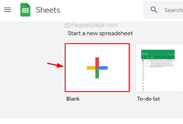
Step 5: Then, click on the Blank option to create a new spreadsheet or select any saved spreadsheet on the google drive listed below.

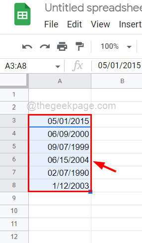
Step 6: If you had selected a blank option then please draft the spreadsheet by entering all the data that are required.
Step 7: Among those data, if you want to change the date values format, then at first you need to select all those cells by clicking on them while pressing and holding the CTRL key.

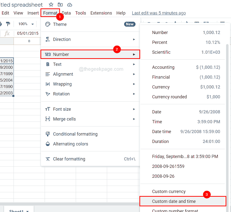
Step 8: After selecting all the cells, you need to go to the Format option on the top menu bar as shown.
Step 9: Then, hover over the Number option from the list and click Custom date and time at the end of the list as shown in the below screenshot.

Step 10: In the Custom date and time formats window, there will be a list of predefined date formats. Please scroll the list and you can select one of them if you want.

Step 11: Otherwise, you can custom change the format. For example, if you want to change the Month format, then click on the Month option as shown below.

Step 12: Select any format that you want from the list for the Month to be displayed in the sheet.

Step 13: If you do not want to see the month in the date format, then simply select Delete from the options which will remove the month option.

Step 14: You can do the same with Day and Year also in the Date format option.
Step 15: Next, if you want to add the time also in the format, then click the More options icon which looks like a down arrow as shown below.

Step 16: Here you can see various options to add in the date format such as Hours, Minutes, AM/PM, etc.
Step 17: Choose any from the shown window.
NOTE: As an example, we have shown only TIME options but you can choose even DATE and DURATION options also as per your requirement.

Step 18: You can also change the hyphen mark character (–) to the backslash symbol (/) also by placing the cursor next to it and changing using the keyboard.
Step 19: Once everything is done, you can click Apply button on top right, which closes the Custom window and you can see all the date values format has been changed.
