Let’s say you have a set of numbers for which you need to find the average. It could be the marks of a list of students, it could be the hits per month of a website, it could be anything. Manually calculating the average values and populating them inside an Excel column is definitely not possible. Well, you need not even think about doing it manually in the first place, when we have a perfect solution that would automate the whole process for you.
Read on, to learn how you can easily find the average of a group of cells in an Excel sheet using a quick formula and to populate an entire column for Average values just with the help of some simple clicks.
Solution
Step 1: Let’s say you have the column named AVERAGE, whose values need to be populated by calculating the average of the numerical values present in each row corresponding to each student.
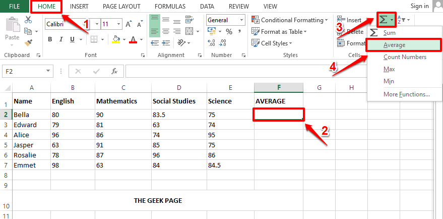
For that, firstly click on the first cell of the column AVERAGE.
Then make sure you are at the HOME tab at the top. As next, click on the dropdown menu associated with the Sigma button and choose Average from the list of options.
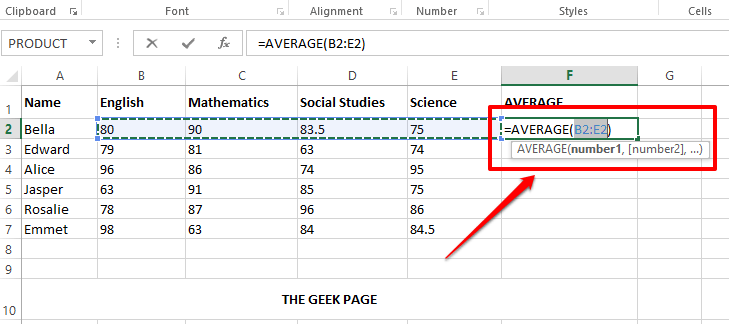
Step 2: Automatically, all the numerical values present in the row, where the selected cell is present, will be considered for calculating the average. In the example screenshot below, the average function is automatically populated as =AVERAGE(B2:E2). Here B2:E2 means all the cells from B2 to E2 in the Excel sheet.
Note: If you need to make any changes, you can always edit the argument list inside the AVERAGE() function. Let’s say if you need to find the average of only C3 and D3 cells, then your Average() function would be =AVERAGE(C3, D3). You can also give static values inside the Average() function as arguments. For example, your Average() function can also be =Average(4,87,34,1).
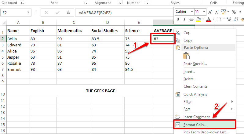
Step 3: Now if you press the Enter key, you can see that the average value is successfully calculated. But the decimals might not be present. If that’s the case, right click on the cell and choose Format Cells from the right click context menu options.
Step 4: In the Format Cells window, make sure you are at the very first tab.
Now, under the Category options, click on Number.
On the right side, enter the number of decimal places you need in the Decimal places filler. I have given 2 in the screenshot below.
Hit the OK button once done.
Step 5: There you are! The average value is now visible with decimal places as well. If you would like to apply the same formula to the rest of the cells in the same column, simply click and drag down the small square-shaped icon at the bottom right corner of your already formatted cell.
Step 6: That’s it. Your formula to find the average of a group of cells is now successfully applied to all the cells present in the same column.
Please tell us in the comments section if you found the article useful.


