There could be multiple occasions where you might want to round off the decimal numbers in your Excel sheet. For example, you might be finding the average marks in various subjects for a student or you might be trying to find the average number of leaves taken by an employee in a year. Whatever be your requirement, the chances of decimal numbers showing up in your Excel sheets are very high.
Though more decimal numbers mean more precision, sometimes, more than precision, the overall appeal of the document matters. Some other times, you just don’t care about 10 decimal places when all you need is just a single number. We totally understand your frustration, and we have a solution too.
Read on, to learn how you can round off decimal numbers in an Excel sheet with the help of some simple steps.
Solution
Step 1: Double click on the cell where you want the rounded-off value to be displayed.
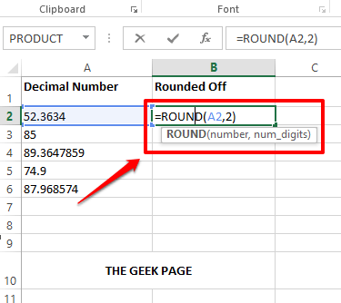
Next, type in =ROUND(<cell id of the cell containing the decimal>,<how many decimal places you need in your final value>). ROUND is a formula function and it takes the above 2 arguments. Replace the arguments with the respective values.
For example, as shown below, my decimal number is in the A2 cell and I need my final value to be rounded off to 2 decimal places. So, my formula would be as shown below.
=ROUND(A2,2)
Note: If you would like to round off the decimal value by 3 decimal places, then in the ROUND function, you need to give the second argument as 3. Example, =ROUND(A2,3). Likewise, you can round your decimal to any number of decimal places as you wish. If you don’t want any decimal numbers at all and just need an integer, then the ROUND function would be =ROUND(A2,0).
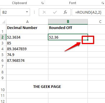
Step 2: If you press the Enter key, you can see that the value has been rounded off by 2 decimal places.
If you would like to apply the same formula to the other cells in the same column, click and drag down the square-shaped icon at the bottom right corner of the cell containing your formula.
Step 3: The following screenshot shows how the ROUND formula is applied to all the cells in the column.
Step 4: If you look at the final value, you can see that there is no uniformity because some numbers do not have decimals, some have only 1 and some have 2. To make the values uniform, select all the cells that you want to format first.
Once the cells are selected, click on the HOME tab at the top. Then click on the Increase Decimal button under the Number section.
Step 5: If you look now, you can see that all the cells have 3 decimal places. Now to make it 2, select all the cells once again and click on the Decrease Decimal button under the Number section itself.
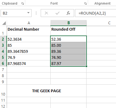
Step 6: There you go! Your decimal values are all rounded off perfectly now and are neatly formatted to 2 decimal places. Enjoy!
Please tell us in the comments section whether you found the article helpful.


