The Strikethrough formatting feature is very useful when you have to ignore something, but the value cannot be deleted altogether. Just like in Microsoft Word, in Excel also, there are many ways using which you can apply the strikethrough formatting to your cells. The strikethrough formatting can be applied to single cells and multiple cells. If you want a particular cell to be struck off based on a specific condition, like in the case of a to-do list, even that is possible!
So what are you waiting for? Dive straight into the article to learn all about the strikethrough formatting feature in Microsoft Excel.
Solution 1: By Using a Keyboard Shortcut
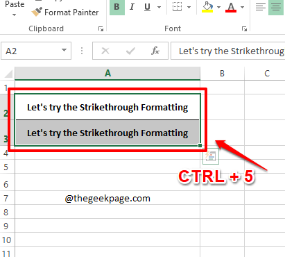
Step 1: Select all the cells that you want to apply the strikethrough formatting to. Once the cells are selected, right click anywhere on the selected area and then press the keys CTRL + 5 simultaneously.
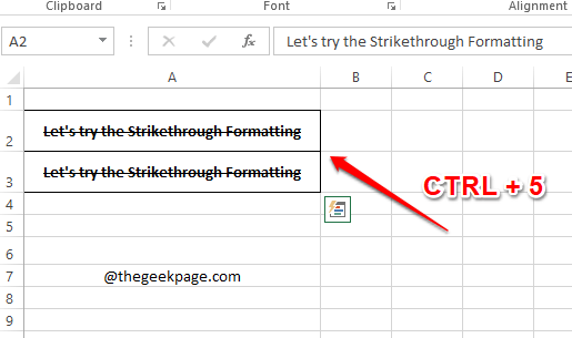
Step 2: Well, that’s pretty much it. Your selected text is now struck off.
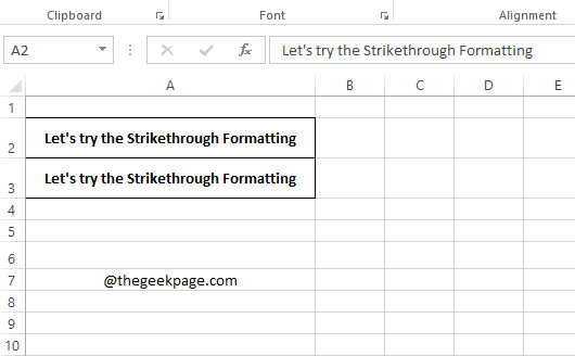
Step 3: If you want to revert the strikethrough formatting, simply select the text again and hit the CTRL + 5 keys again. Yes, CTRL + 5 is your personal toggle switch for strikethrough from now on, indeed!
Solution 2: By Adding Strikethrough Option to Quick Access Toolbar
The quick access toolbar is located at the very top of your Excel window, even above the tabs ribbon. You can easily add a shortcut for Strikethrough on your quick access toolbar and thus it can be used very easily every time you need to apply the strikethrough formatting in your document.
Step 1: Right click anywhere on the quick access toolbar at the topmost position in your Excel window. From the right click context menu options, click on Customize Quick Access Toolbar.
Step 2: When the Excel Options window launches open, on the left pane of the window, click on the Quick Access Toolbar first.
Now on the center pane of the window, click on the dropdown menu associated with Choose commands from option and choose the option All Commands.
From the list of commands underneath All Commands, scroll down and click on the one that says Strikethrough.
Hit the Add button as shown in the screenshot below.
Step 3: Now you can see that the Strikethrough option is added to the section on the right pane of the window.
Hit the OK button.
Step 4: That’s it. The Strikethrough option is now added to your quick access toolbar.
Step 5: Select the text that you want to strike off and then hit the Strikethrough quick access, that you added to your quick access toolbar.
Step 6: Well, that’s it. Your text is well struck off! It is indeed a job done in a single click! Enjoy!
Wondering how it is a single-click job? Well, adding the Strikethrough formatting option to the quick access toolbar indeed takes some steps, but once it is added, it is added forever.
Solution 3: Using the Format Cells Options
Step 1: Select all the cells that you want the strikethrough formatting to be applied to and then right click anywhere on the selected region.
From the right click context menu, click on the Format Cells option.
Step 2: On the Format Cells window, make sure you are at the Font tab first.
Now, under the Effects section, check the checkbox corresponding to the Strikethrough option. Remember, the checkbox has to be checked with a tick mark itself, and not with a dot or anything else.
Once done, hit the OK button at the bottom.
Step 3: That’s it. Look at the screenshot below. Isn’t it exactly what you wanted?
Solution 4: Strikethrough Using Conditional Formatting
This is a very useful solution if you have to apply the Strikethrough formatting to your cells based on some conditions. Say, for example, you have a to-do list in one column and the status of each item of the to-do list in another column. If the status says Done, then the corresponding to-do list item has to be automatically struck off. This is basically the dynamic formatting of cells. Let’s see how this can be done easily.
Step 1: Firstly select all the cells that you want to add the conditional formatting to.
Then click on the HOME tab at the top.
Now under the HOME tab options, click on the dropdown Conditional Formatting and then click on New Rule.
Step 2: A new window named New Formatting Rule will now launch before you. Under the section Select a Rule Type, click on the very last option, which is, Use a formula to determine which cells to format.
As next, under the section Edit the Rule Description, we need to define the rule. The return value of the rule can only be either true or false.
In the example below, the rule I have defined is as follows.
=&B2 = "Done"
The rule simply says that, lock the value B and keep the value 2 changing, so that all the values in the Status column are checked against the word Done. If there is a match, then the formatting that we define in the step below has to be applied to the cell under processing. You can apply any rule as you wish. But remember to enclose constant string values inside double-quotes.
As next, let’s apply the Strikethrough formatting, for that click on the Format button.
Step 3: On the Format Cells window, click on the Font tab first.
Under the section Effects, check the checkbox corresponding to the option Strikethrough. Make sure the checkbox has the tick mark.
Hit the OK button.
Step 4: That’s it. Hit the OK button.
Note: The rule is applied to all the cells in the selected range of cells. Each cell is taken and the rule is checked.
Remember, the rule can only return 2 values; true or false. If the result of the rule is true, then the formatting that you define gets applied to the cell.
Step 5: Viola, you now have conditional striking off formatting applied to your selected cells.
Now if you change the value in the Status column from Not Done to Done, then the corresponding value in the To-Do List column will be struck off. Job well done!
Hope you had fun reading the article. Don’t forget to tell us which method is your favorite. Our favorite is the last method, as it is very dynamic.
Stay tuned for more amazing tricks, tips, and how-to articles.


