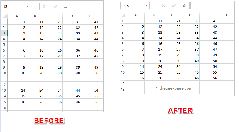
No one has an argument when it comes to blank rows in excel sheets. Of course, they are a huge nuisance. Collecting data from an excel file that has blank rows can lead to errors. If there are any automation procedures involved, definitely blank rows are going to give a lot of trouble. At any cost, everyone wants the blank rows gone, that too, with minimal steps possible.
So how can you quickly get rid of these problem makers? Well, we are not going to give you a single solution for this, instead, we are going to give you 5 solutions, from which you can pick your favorite!
Read on, to learn how you can easily delete blank rows from your Excel sheets, with the simplest of the steps, through 5 different methods.
Solution 1: By Manually Selecting and Deleting Blank Rows
We know no one like anything manual and that it’s all automation these days. But if there are only a couple of blank rows to be deleted, then manual deletion sure is something you can consider.
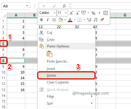
To manually delete the blank rows, firstly, hold down the CTRL key. Keep the CTRL key pressed and click on the heads of the blank rows that you want to delete. You can even select other unwanted rows, they need not be blank to be deleted.
Once all the rows to be deleted are selected, simply right click and click on the Delete option. That’s it, all of the selected rows would now be deleted.
Solution 2: Using Go To Special Feature
The Go To Special feature is useful for many purposes. But today, we are going to use it to hunt down the blank rows in your excel and to delete them all at once.
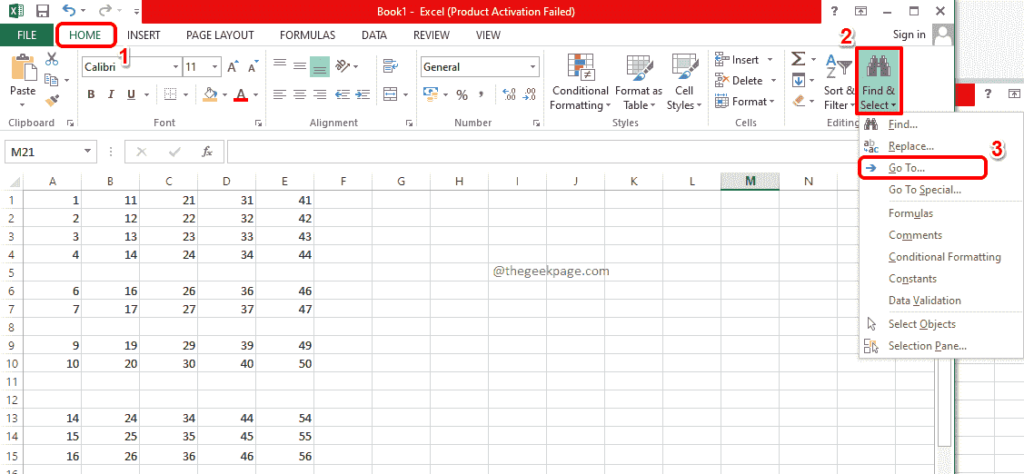
Step 1: Firstly, make sure you are at the HOME tab of your excel sheet. As next, towards the right corner of the window, find and click on the Binocular icon for Find and Select and choose Go To from the dropdown menu.
Step 2: In the Go To window, click on the button named Special.
Step 3: Choose the radio button corresponding to Blanks and hit the OK button.
Step 4: If you now look at the excel sheet, you can see that all the blank rows are selected automatically.
To delete them, either you can right click somewhere and hit the Delete option.
Or you can click on the Delete button at the top ribbon as shown in the screenshot below.
Step 5: There you are! All your blank rows are now gone!
Solution 3: Through Filter Method
In this method, we are going to filter out your columns based on blanks rows and then delete the results that we obtain.
Step 1: Firstly, click on a column header that has blank rows present. Next, make sure you are on the HOME tab.
Now, find and click on the button that says Sort & Filter. This button is present at the top right corner of your Excel window.
From the dropdown list, click on the Filter option.
Step 2: Now you will have a dropdown arrow associated with the column you chose. Click on this dropdown arrow to apply the filter.
Step 3: As next, check the checkbox corresponding to only Blanks and then hit the OK button.
Step 4: Now you will be shown only those rows that are blank. You can identify this by the blue number marking on row headers. Drag and select all of them. And then click on the Delete dropdown list on the top ribbon and then finally hit the Delete Sheet Rows option.
Step 5: To view the other rows that have data, let’s remove the filter we applied. For that, once again click on the Sort & Filter dropdown from the top ribbon and then click on the Filter option. This will disable the filter.
Step 6: That’s it. You now have the final rows that are not blank.
Solution 4: Through Sorting Method
This is another easy method where you sort the entire excel sheet and push the empty rows to the bottom so that they can be just ignored.
Step 1: Select any column that has blank values, by clicking on the column header.
In the example below, clicking on E selects the entire column.
Once you have selected the column, make sure you are at the HOME tab. Then click on the Sort & Filter dropdown menu and finally click on the Sort Smallest to Largest option.
Step 2: When you get the Sort Warning dialog box, choose the radio button corresponding to the option Expand the selection and then hit the Sort button to sort the sheet.
Step 3: The sorted sheet would have all the blank rows pushed to the bottom and you can just ignore them.
Solution 5: Using Find and Replace Functionality
This method is very similar to the Go To Special method. In this method also, we find the empty rows and then delete them all at once.
Step 1: Press the keys CTRL + F at the same time to bring up the Find and Replace window.
When it comes up, click on the button named Options >>.
Step 2: Leave the Find what text box empty.
From the dropdown menu associated with the option Within, choose Sheet.
Also, for Look in dropdown menu, choose Values.
Check the checkbox for the option Match entire cell contents.
Finally, click the Find All button.
Step 3: The previous step would return all the empty rows in its search results section.
Click on one of the search results and then press the keys CTRL + A simultaneously to select them all. You can now hit the Close button for Find and Replace window to close it.
If you now look at the excel sheet, you can see that all the blank rows are selected and highlighted.
Step 4: Now as usual, either you can right click somewhere and click on the Delete option from the right click context menu or you can click on the dropdown button Delete and choose Delete Sheet Rows to delete all the selected blank rows all at once.
All the methods listed in this article are simple, but our personal favorite is Method 4, the sorting method. Do you have a favorite too? Please tell us too, in the comments section.
Hope you found the article useful.


