Many times you might end up with huge Excel files with lots of balances and due dates. You might need to find some way to highlight all those customers who should pay their amount dues, to avoid late fee charges. In such cases, it would be really handy if you can apply a rule to your Excel sheet to highlight those balance amounts. In this article, we explain in some simple steps how you can easily get this task done. Hope you enjoy reading!
Sample Data
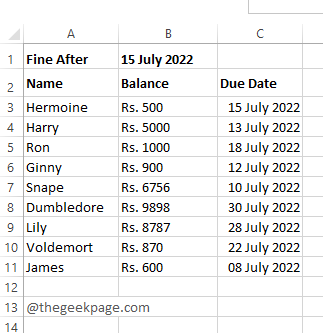
Let’s say you have the following sample data. In column Name, you have the names of your customers. In column Balance, you have the balance amounts to be paid by them and in Column C, you have the due dates corresponding to each customer.
At the top of the table, you have a cell, B1, inside which you have the date after which the fines are to be collected. That is, for each customer, if their due date value is lesser than the date value present in B1, then they have to pay their respective balance amount to avoid fines.
Our requirement is to highlight the balance amount if it is to be paid to avoid fines.
Solution
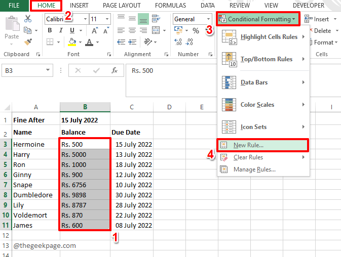
Step 1: Firstly, select the values in the column, Balance, that you want to be highlighted.
After that, click on the HOME tab and then click on the Conditional Formatting dropdown button.
From the list of options, click on New Rule.
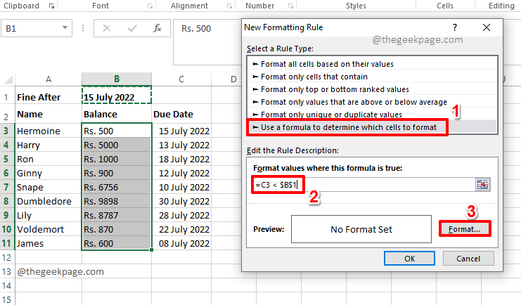
Step 2: On the New Formatting Rule window, under the Select a Rule Type section, click on Use a formula to determine which cells to format.
Now under the Edit the Rule Descriptions field, type in your formula.
Since I want to highlight the cells in the Balance column based on date dependencies, as mentioned in the Sample Data section above, I have formed my formula as follows.
=C3 < $B$1
Note: We need to check all the values in the Due Date column against the Fine After date, which is present in cell B1. Hence, C3 should be varying and B1 should be constant. That’s why we have put $ symbol for the B1 cell, to keep it constant.
Once you are all done with the formula part, let’s get to the formatting part. For that, click on the Format button.
Step 3: You can choose any formatting as per your choice. Since I want the cells to be highlighted, I have gone to the Fill tab first.
Then I have chosen a color. The sample preview can be seen under the Sample section. Once you are all done, hit the OK button.
Step 4: When you are back at the New Formatting Rule window, hit the OK button.
Step 5: That’s it. All the cells in the Balance column that have balance due are now automatically highlighted.
Please tell us in the comments section if you have any concerns regarding any of the steps. We are always here to help.
Stay tuned for more cool tricks, tips, how-to articles, and hacks.


