Sometimes when you copy data from one Excel sheet to another or when you import data, some space characters could make unwanted visits to your new sheet. They could be everywhere. Sometimes to the left of your actual data, sometimes to the right. Wherever they come, they are indeed a huge inconvenience and they do make your Excel sheet look unprofessional. So, is there a way how you can effectively and efficiently remove the unwanted space characters in your Excel document? Of course, there definitely is!
Here in this article, we have detailed how you can easily remove unwanted space characters from your Excel sheet, with the help of some simple examples. So what are you waiting for? Let’s dive into the article.
Solution 1: How to Remove Unwanted Spaces when there are No Space Characters between Data in a Column
This solution can be applied only if there are no space characters between the data and there are space characters to the left and/or to the right of the data. In such cases, a simple solution works perfectly, and let’s see how it is done.
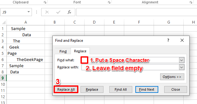
Step 1: Let’s say you have a column as shown in the screenshot below. In this column, there are space characters to the left of the data in some cases, and to the right of the data as well, in some other cases. Also, there are no space characters between the data in any of the cells.
In such cases, press the keys CTRL + H to bring up the Find and Replace window. In the Find what field, put a single space character. Leave the Replace with field empty. Then click on the Replace All button.
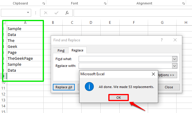
Step 2: This would replace all the space characters found in your Excel sheet with empty characters. Hit the OK button to close the replacements confirmation window.
That’s it. Your data is now well formatted with no space characters before and after the data in each cell.
Solution 2: How to Remove Unwanted Spaces when there are Space Characters between Data in a Column
Now let’s take cases where there could be space characters to the left, to the right, and in between the data as well. In such cases, if you use the Find and Replace method detailed in the solution above, the space characters between your data would also get replaced and your data would be corrupted. So, if there are space characters between your data, you need to follow the solution detailed below.
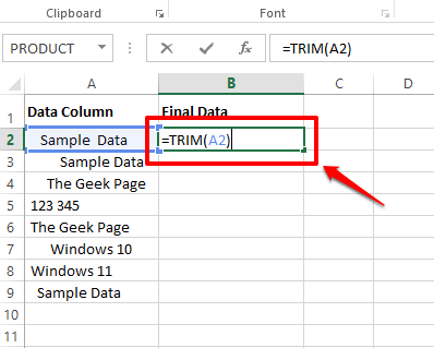
Step 1: For this solution, we are going to make use of a formula function named TRIM. Create a new column for the new space-formatted data.
Now, click on the first cell of the new column and write down the formula as =TRIM(A2). If your data to be formatted is in a different cell, you need to replace A2 with the cell id of the cell that has the data to be formatted.
Step 2: Now, if you hit the Enter key or click elsewhere, your data would be trimmed of spaces to the left and to the right, whereas the space characters within the data would be retained.
To apply the same formula to all the cells in the same column, click on the small square shape at the bottom right corner of the cell containing your formula and then drag it down.
Step 3: There you go! Your formula is now successfully applied across the column.
Step 4: Now you have 2 columns, one with the non-formatted data and another with the final formatted data. Just don’t delete the non-formatted data column yet. If you do, you will get the following reference error.
This happens because your final formatted data column has references to your non-formatted data column. So how do you go about deleting the source column? Definitely, you do not want 2 columns in your Excel.
For that, right click on your formatted column and hit the Copy option.
Step 5: Now click on the header of the source column that is non-formatted and you want to be deleted.
Step 6: Right click anywhere on the selected column and then hover over the Paste Special option. From the Paste Special options, click on the first option available under the Paste Values section.
This would copy the values only, and not the formula, leaving no references.
Step 7: Now you have 2 columns. The first one with no formula references and dependencies and the second one, with references. So you can simply delete the second one.
For that, right click on the column header of the column to delete and click on the Delete option. Enjoy!
If you are stuck at any of the steps, please do drop a comment, we would be happy to help. Stay tuned for more amazing tricks, tips, and how-to articles.


