Both Google Sheets and Excel are powerful tools. Google Sheets are most widely used when you are working globally often sharing data with others. It is very useful for collaboration purposes. Meanwhile, Excel is used offline most of the time for your own calculations, etc. Suppose you are using Google sheets all the time and need to take a backup, you will download it and save it on your computer. But imagine you are working on some data analysis project and you are doing a lot of changes in the Google sheet. Every time you do the change you have to download it for backup. This becomes a tedious task, isn’t it? There is a way to make things simpler. You don’t need to download the Google sheets every time when there is an update but still, you will have the latest data backup on your computer. Thinking how is it possible? In this article, we will learn how to do it that is how to connect and synchronize Google Sheets to Excel.
Steps To Connect Google Sheets To Excel
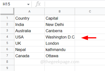
Step 1: Open the Google sheets that you want to connect to excel. Make sure you have some data in the Google sheets. Here I have a sample list of data and countries and capitals.
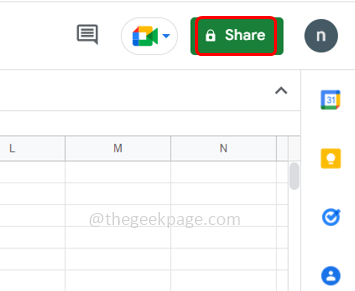
Step 2: Click on the Share button which is at the top right corner.
Step 3: If you have not named the google sheet, you can name it now. Or if you do not want to name it click on skip. If it is already named then continue with Step 4
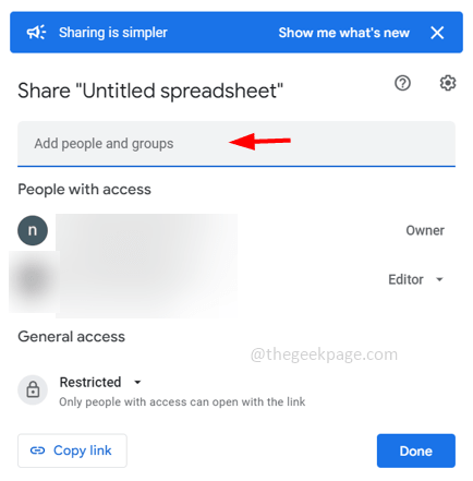
Step 4: You will get a pop-up that has a link. Now you have to choose the access either Restricted which means only people with access can view the data with the help of a link or choose Anyone with the link which means anyone on the internet with the link can view the data
Step 5: If you are selecting Restricted then to add people, you can type the email ids of the people in the Add people and groups field
Step 6: Here I have selected Anyone with the link and click on the Copy link to copy it and then click on Done
Step 7: Now create Microsoft Excel Worksheet. To do so, go to the location on your computer where you want to create the Excel, right-click on the blank space, and click on New
Step 8: Choose Microsoft Excel Worksheet from the list. A worksheet will be created.
Step 9: You can give it a name. Open the excel worksheet
Step 10: Go to the Data tab from the excel ribbon at the top and click on from web. If you do not find it click on Get Data
Step 11: Select From Other Sources and from the fly-out list click on From web
Step 12: In the appeared window paste the copied link in the URL field
Step 13: Move to the end of the link and remove all the characters from the edit till the last
Step 14: And replace those removed characters with the export?format=xlsx
Step 15: Now the link looks like below. Click on OK
Step 16: Click on Connect
Step 17: A navigator window will be opened which will have the google sheets on the left side. When you click on the sheet, on the right side you can see the preview of the data that you had in the google sheet. But the Column headers and not as expected.
Step 18: To change the Column headers, click on Transform data at the bottom and the data will be loaded to the Power Query Editor
Step 19: Choose the Transform tab, click on Use first row as headers dropdown and choose Use first row as headers
Step 20: Now you can observe the headers have been changed. To load the data into the excel worksheet, click on the Home tab at the top
Step 21: Click on Close & Load which is at the top left corner
Step 22: It will take a few seconds and the data will be loaded into the Excel worksheet. You can also see the number of rows loaded and the name of the worksheet on the right side of the Excel
Steps To Synchronize The Data InTo Excel
Now that you have connected and loaded the data present in the google sheets to excel, let us see if there are any modifications or updates made in google sheets, how it reflects in excel immediately.
Step 1: Here, I have added a few more data in the Google Sheet and saved it
Step 2: Excel should also get updated with the latest data. So back in the excel worksheet click on Refresh and the latest data will be updated
Step 3: Instead of clicking on the Refresh button every time, you can auto-update the worksheet at regular intervals. So select the table or click on any cell in the table and click on the Refresh All dropdown button.
Step 4: Choose Connection Properties
Step 5: Query properties window will appear, tick the checkbox beside refresh every by clicking on it and specify the time for the refresh to take place. It is in minutes.
Step 6: Also click on the checkbox beside Refresh data when opening the file to enable it and click on OK to save the changes
Step 7: Save the Excel Workbook and close it
Step 8: Now add some more data in the Google sheets and save it
Step 9: Open the excel workbook and if you get any security warning at the top, click on Enable and wait for a second to run the background query
Step 10: And it’s done, the latest data is seen in excel without any clicks.
That’s it! I hope this article is helpful and you got it done easily. Thank you!!


