How To Hide Sheets, Gridlines And Cells In Excel Sheets:- Are you looking for ways to hide Sheets, Gridlines or Cells in your excel sheet? You are in the right place. We have got the perfect results for all your queries. Dive into the article to learn how to hide sheets, gridlines and cells in excel sheets.
Steps To Hide Sheets In Excel
STEP 1
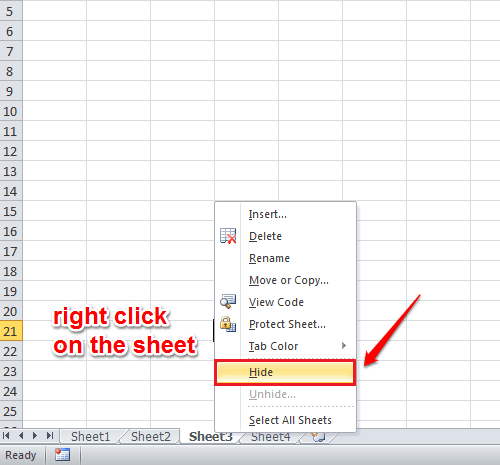
- Right click on the sheet that you want to hide in Excel. Now from the context menu that appears, find and click on the Hide option.
STEP 2
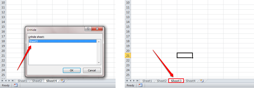
- You can’t see a hidden sheet. So to unhide a hidden sheet, right click on a visible sheet. As next, click on the Unhide option from the context menu that appears.
STEP 3
- This will show all the hidden sheets in a small window. Simply select the ones that you want to unhide and click Ok button. If you check now, you can see that the hideen sheet is visible.
How To Hide Gridlines In Excel
STEP 1
- You might want to take off the gridlines from the Excel sheet. For that, open the excel sheet that you want the gridlines to be removed from.
STEP 2
- As next, click on the View tab. Now uncheck the checkbox corresponding to Gridlines. And the gridlines are gone!
How To Hide Cells In Excel
STEP 1
- Select the cell that you want to hide and right click on it. Choose Format Cells option from the context menu.
STEP 2
- A new window named Format Cells opens up. Click on the Number tab. Under Category section, choose Custom option. Now for type, give ;;; without any spaces. Refer to the following screenshot if you have any doubts. Hit OK once you are done.
STEP 3
- Now if you look at the content of the cell, you can see that it is hidden. But if you look at the fomula tab above, you can see the content there, so no worries. To revert back, simply set the Type to General in the Format Cells window.
Try out the excel hiding tricks today itself. If you have any doubts regarding the article, please feel free to leave comments. We would be happy to help. Stay tuned for more tricks, tips and hacks.


