How To Format Text In Microsoft Excel Using UPPER, LOWER & PROPER Functions:- Forget deleting all the text just because you forgot to enter in its proper format. Now you can type in the text in any way you are comfortable with and later format the text with three simple functions; the UPPER, the LOWER and the PROPER functions. Dive into the article to learn all about this simple trick.
STEP 1
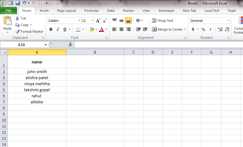
- Open the sheet in Excel which has unformatted text. Let’s say you want it to be Properly formatted. That is, you want the first letter of every word to be capitalized and the rest in small letters.
STEP 2
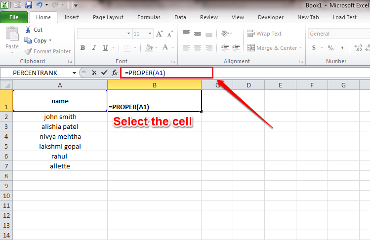
- For that, click on the cell adjacent to the top most cell of your unformatted column. That is, if the unfomatted text starts at cell A1, you should click and select the cell B1. Now in the formula bar, type in =PROPER(A1). Once you are done, hit Enter key.
- Note : A1 and B1 cells are given as examples. You can choose any cells as long as they satisfy the conditions of being adjacent to each other and are in the same row. Otherwise, you won’t be able to apply the formula rule to the rest of the column.
STEP 3
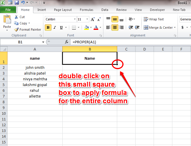
- Now simply click on the small square box at the bottom right corner of the new cell. This will apply the formula rule to the entire column.
STEP 4
- There you are! You have successfully applied the formula rule to the entire column. As next, let’s get rid of the first column which is unformatted. For that, simple copy paste won’t be enough as this will give formula error. Follow the steps below to overcome this issue.
STEP 5
- Copy the contents of second column by right clicking and choosing copy. Or you can use the key combination of CTRL+C.
STEP 6
- As next, choose the entire first row. You can do this by clicking on the cell head, that is, A in our case. Now right click and choose Paste Special. From the options in Paste Special, pick Paste Values. You can click on the first option in the Paste Values entries. That’s it. Refer to the screenshot given below for reference.
STEP 7
- Now you can see that the values in the second column is successfully cloned to the first one.
STEP 8
- At this stage, you can easily get rid of the second column by clicking on its cell head, B and hitting Delete key.
STEP 9
- You can also try capitalizing the entire text. For that, the function used is UPPER function. Just like before, click on the adjacent cell and in the formula bar, type in =UPPER(A1).
STEP 10
- Again, click on the small square to apply the formula column wide.
STEP 11
- Next one is turning the entire text into small letters. For that, the function used is LOWER function. Just like before, click on the adjacent cell and in the formula bar, type in =LOWER(A1).
STEP 12
- Click on the small square to apply the formula column wide. Yes, we are done!
Hope you found the article useful. Please leave comments in case if you have any doubts. We would be happy to help. Stay tuned for more tricks, tips, and hacks.


