As we all know Office 365 comes with Excel 365 bundled with it. Microsoft has added various new features to Excel 365. One such feature is Dynamic Array Formulas. Usually, the formula would return only a single value as a result to a cell. But now, with this new feature in place, multiple values can be returned.
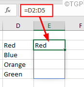
For example, in Excel 2019 and earlier versions let’s say you apply the formula =D2:D5 on the cell, the result would be limited to the first cell.
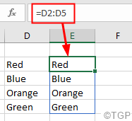
When we had to apply the formula on all the corresponding cells, we made use of Array notation(Ctrl+Shift+Enter). However, in Excel 365 it is not so. When you apply the same formula, automatically the values are spilled onto all the corresponding cells. Refer to the below image, for more details.
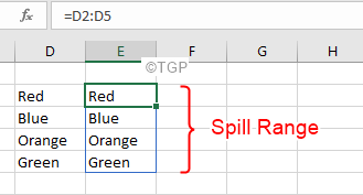
The area of cells in which the result is spilled into is called Spill Range. Refer to the below image
NOTE:
- The Spill is Automatically enabled with Dynamic Arrays(Currently this feature is supported only in Excel 365) and the feature cannot be disabled.
- The Spill feature is enabled on all the formulas with or without functions.
Spill Errors are seen when the formula is intended to return multiple values, however, the results cannot be put on the cells. The error looks as follows :
Possible reasons to encounter #SPILL Error are :
- The Spill range contains some value because of which the results cannot be populated in the cells
- The Spill range has merged cells.
- When old sheets(created using Excel 2016 or earlier) with formulas supporting the implicit intersection are opened in Excel365.
- When you apply the dynamic array formula on an excel table.
If you are seeing the #SPILL error in excel, then do not worry. In this article, we will be demonstrating different ways to identify the root cause for this issue and also look at ways to fix the #SPILL error
Identify what is causing the #SPILL error
When you see a spill error, first check why you are seeing the error, to do so,
Step 1: Click on the cell that shows #SPILL! error
Step 2: Click on the Exclamation mark as shown below
Step 3: The First line tells us what is causing the Error. For example, in this case, the error is seen as the Spill range isn’t blank
Fixes to be followed when Spill range isn’t blank
Follow the below fixes when you see that the Spill range isn’t blank
Fix 1: Delete the data that is blocking the Spill range
If there is some data already within the cells in the Spill range, you will see an #SPILL error on applying the formula.
When you can clearly see the data that is blocking the Spill range
Consider the below example, When you apply the formula =D2:D5 on the data, a SPILL error is thrown as there is I m here within the spill range.
In order to get rid of the #SPILL error just move the data or delete the data from the spill range.
When the data blocking the Spill range is hidden
In some cases, the data that is blocking the Spill range is hidden and not very obvious as seen in Case 1. Consider the below example,
In such cases, to find the cell that is blocking the Spill range, follow the below steps:
Step 1: Click on the cell that shows #SPILL! error
Step 2: Click on the Exclamation mark as shown below, You can see that the error is because the Spill range isn’t blank.
Step 3: From the drop-down, click on Select Obstructing Cells
Step 4: The cell that is blocking the Spill range is highlighted as shown below
Now, that you know which cell is blocking, check what exactly is causing the issue.
Step 5: On careful examination of the cell, you can see some data hidden within the cells.
As seen in the above image, there is some data. Since the font has a white color, it isn’t easy to recognize the blockage. In order to get rid of the error, delete the data from the cell within the Spill range.
Fix 2: Remove the Custom Number formatting ; ; ; applied on the cell
At times, when a custom number formatting ; ; ; is applied on a cell, there are chances to see the SPILL error. In such cases,
Step 1: Click on the cell that shows #SPILL! error
Step 2: Click on the Exclamation mark as shown below.
Step 3: From the drop-down, click on Select Obstructing Cells
Step 4: The cell that is blocking the Spill range is highlighted as shown below
Step 5: Right-click on the obstructing cell.
Step 6: Choose Format Cells
Step 7: Format Cells window opens. Go to the Number tab
Step 8: From the left-hand pane, select Custom
Step 9: From the right-hand side pane, change the Type from ; ; ; to General
Step 10: Click on the Ok button
Fix to be followed when Spill range has merged cells
If you see that the error is because the Spill range has merged cells as shown below,
Step 1: Click on Select Obstructing Cells from the drop-down
Step 2: The Obstructing cell will be highlighted
Step 3: Under the Home tab, click on Merge & Center
Step 4: From the drop-down, select Unmerge Cells
Fix to be followed when Spill range in the table
Dynamic array formulas are not supported in Excel Tables. If you see the #SPILL error on an excel table as shown below with the message Spill range in table,
Step 1: Select the table completely
Step 2: Click on the Table Design tab from the top menu bar
Step 3: Choose Convert to Range
Step 4: You will see a confirmation dialog popping up, click on Yes
Fix to be followed when Spill range is out of memory
When you are trying to identify the cause of the #SPILL error, if you see that the error states Out of Memory, then that is because the dynamic array formula you are using references a large range, in such cases, excel runs out of memory causing Spill error. To overcome the error, one can try referencing a smaller range.
Fix to be followed when Spill range is unknown
This error is seen when the size of Spilled Array changes and excel is not able to establish the size of the Spilled range. Generally, when you use random functions like RANDARRAY, RAND, or RANDBETWEEN along with Dynamic Array functions such as SEQUENCE this error is seen.
To understand it better, consider the below example, lets say the function SEQUENCE(RANDBETWEEN(1,100)) is used. Here RANDBETWEEN generates a random integer that is greater than or equal to 1 and less than or equal to 100. And SEQUENCE generates sequential numbers(Eg-SEQUENCE(5) generates 1,2,3,4,5). However, RANDBETWEEN is a volatile function and keeps changing its value every time an excel sheet is opened or changed. Because, of this, the SEQUENCE function will not be able to determine the size of the array that it has to generate. It wouldn’t know how many values to generate and thus throws a SPILL error.
When you are identifying the cause for the error, you see Spill range is unknown
In order to fix this kind of error, try having a different formula that suits your need.
Fixes to be followed when Spill range is too big
Let’s say you are identifying the cause and you notice that the error is seen because the Spill range is too big as shown below.
When Dynamic Array was not in place, there was something called implicit intersection in excel that forced to return a single result even when the formula had a potential of returning multiple results. Consider an example, if the formula =B:B*5% is applied on Excel 2019 or earlier versions, with the implicit intersection in place, the result would be as follows:
However, when the same formula is used in Excel 365, you see the following error
In order to solve this, try the following fixes
Fix 1: Apply implicit intersection using @ operator
When we say =B:B, the dynamic array will reference the whole of the B column. Instead, we can force excel to impose implicit intersection using @ operator
Change the formula to =@B:B*5%
Because the implicit intersection is added, the formula will be applied to a single cell. In order to extend the formula,
1. Just click on the dot as shown below
2. Drag it down onto the cells as required. This will apply the same formula to these cells.
Fix 2: Instead of referring to the column, refer to the range
In the formula, =B:B*5% , we are referring to column B. Instead refer to a particular range, =B2:B4*5%
That’s All
We hope this article has been informative.
Kindly like and comment if you were able to fix the issue with the above methods.
Thank you for Reading.


