How to Count the Number of Cells Containing Text Strings in Excel

If you are searching for a way to count the cells containing only text characters in your Excel sheet, well, we have got happy news for you, you can’t be at a better place. This Geek Page article is all about text strings and how to count the number of cells containing them. We have added some extra cookies, by detailing on methods, using which you can easily add up some more conditions to your text string counting. Well, what are you waiting for? Let’s jump in, shall we?

Read on, to learn how you can return the number of cells containing text strings in your Excel sheet, by using some simple inbuilt formulae. The article also explains in detail the COUNTIFS formula, which lets you specify more than one criteria to count your cells. Hope you find the article useful.

Example Scenario

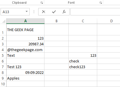
We have the following sample table that has various values. Some cells contain only text-only values, some contain only numeric values, some only date values, etc. Some cells are even blank, some a combination of different data types. Let’s see how we can effectively count the cells containing text values, in the following sections.

 

 

Section 1: Count the Number of Cells Containing Any Text Sting Using COUNTIF Function

In this section, we explain in detail how you can count the number of cells in an Excel sheet, that contains any kind of text inside them.

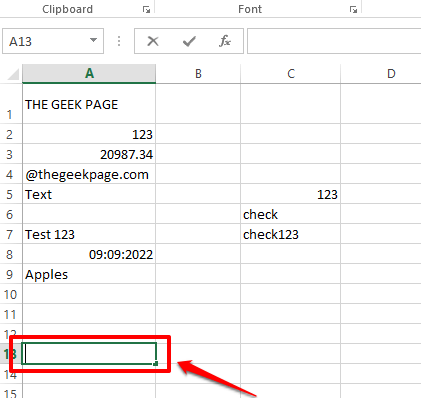
Step 1: Firstly, double click on any cell. This is the cell where the result value will be generated. That is, this is the cell where we will define the formula to count the number of cells containing text values.

Just remember that the selected cell needs to be outside the range of cells that you need to count.

 

 

Step 2: As next, inside the selected cell, type in or copy and paste the following.

=COUNTIF(

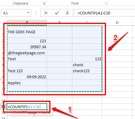
Now, we need to define the range. either you can type in the range of cells or you can simply drag and select the range of cells from your Excel sheet.

 

 

Step 3: Once the range is selected, put a comma and then type in “*”). Don’t forget to close the bracket. So the final formula should be in the following format.

=COUNTIF(range,"*")

The formula as per the example screenshot below is as follows.

=COUNTIF(A1:C10,"*")

 

 

Step 4: That’s it. If you hit the Enter key now, the COUNTIF function would return the total number of cells containing text values inside them.

In the example below, the total number of cells is 7. In green, all the cells containing text strings are marked, and only these cells are counted. Blank cells are not counted.

 

 

Formula Explanation

The COUNTIF function takes in 2 arguments. The first argument is the range of cells and the second argument is the criterion to count. In the example above, we have given “*” as the second argument, which results in the COUNTIF function counting all the cells, mentioned in the range argument, containing any text values.

Section 2: Count the Number of Cells Containing Any Text String Using SUMPRODUCT Function

The SUMPRODUCT function also returns the number of cells containing any text string, from the selected range of cells. The end results of both the SUMPRODUCT function and COUNTIF function, mentioned in the section above, would be the same, but the way they work internally is different for both.

Step 1: Double click on any cell, where you want the final result to be populated at. Now, copy and paste the following formula.

=SUMPRODUCT(--ISTEXT(range))

The range value should be replaced with the actual range of cells that you want to checked. You can either type in the range manually or you can open the ISTEXT function brace, and then drag and select the range of cells just like how you did it in the section above. Once the range is entered, don’t forget to close the brace.

In the example below, I have replaced the range in my formula and the final formula in my case is as follows.

=SUMPRODUCT(--ISTEXT(A1:C9))

 

 

Step 2: That’s it. If you hit the Enter key, you can see the final count, just as simple as that.

 

 

Formula Explanation

1. This method uses both the SUMPRODUCT formula and the ISTEXT formula to calculate the final result. As ISTEXT function is enclosed inside the SUMPRODUCT function, ISTEXT function gets calculated first.
2. ISTEXT function takes in the range of cells as its argument. So each cell in the given range is checked for text values. If the cell contains a text value, then the ISTEXT function returns the value true. Else the value false is returned.
3. Now, since ISTEXT function is taking a range of cells and not just a single cell, it returns an array of true and false values. So our ISTEXT function would return something like {true, false, false, true, true, false, true, false, true…..}
4. Now coming to the — inside the =SUMPRODUCT(–ISTEXT(A1:C9)) formula. — is applied to all the values inside the array returned by ISTEXT. It converts true values to 1 and false values to 0.
5. Now, finally, the SUMPRODUCT function would return the sum of all 1 values, which in effect is returning the total number of cells containing a text value.

Section 3: Add More Criteria While Counting the Cells Containing Text Strings Using COUNTIFS Function

Now let’s say you have to get the total count of all the cells in your sheet that have text values inside them, but you do not want the cells that contain a specific text to be counted, say, for example, “Apples“. In such cases, where you want to add more conditions to your COUNTIF function, you can reply on the enhanced version of COUNTIF, which is COUNTIFS.

In the following steps, we have explained in detail how you can make the best use of the COUNTIFS function.

Step 1: Double click on the cell where you want the final result to be visible. Now, copy and paste the following formula onto it.

=COUNTIFS(range,"<first_condition>",range,"<second_condition>")

Replace range with the actual range of cells. Please remember to give the same range in both places, otherwise, you might get an error.

Please refer to the following screenshot for an example, where range values and the conditions are replaced.

=COUNTIFS(A1:C12,"*",A1:C12,"<>Apples")

 

 

Step 2: Hitting Enter key would give you the desired result. Wondering what happened? Head on to the Formula Explanation section.

 

 

Formula Explanation

1. The formula in the example scenario is =COUNTIFS(A1:C12,”*”,A1:C12,”<>Apples”).
2. The first condition inside the COUNTIFS function, which is “*”, takes the count of all the cells containing text strings.
3. The second condition, which is “<>Apples”, takes the count of all the cells whose value is not equal to Apples.
4. So, combining the first and second conditions, we get the total number of all the cells that contain text values, but the text value shouldn’t be Apples. This means the word Apples is not considered as a text anymore because of our second criterion.

Section 4: Count the Number of Cells Containing Partially Matched Text Strings

In the section, let’s discover how you can get the count of cells containing a string that you specify.

Step 1: Let’s say you want to get the count of all the cells that contain the word Apples. For that, double click on the cell where you want the count value to be displayed.

The generic version of this formula would be as follows. Copy and paste it onto the selected cell.

=COUNTIF(range,"<keyword>*")

Note: Replace range and keyword values in the formula, but make sure to put the asterisk after the keyword.

We have replaced the range value and the keyword value in the following example.

=COUNTIF(A1:C12,"Apples*")

 

 

Step 2: Hit the Enter key to view the result value.

 

 

Formula Explanation

The COUNTIF formula, in this case, takes in 2 arguments. The first value is the range of cells to be checked for and the second argument is the keyword that needs to be present in the text string. The asterisk(*) character ensures that the cell is counted only if the value inside it starts with the keyword that we specify. If you are ok with counting the cell even if the keyword comes at the end of the word inside the cell, then you need to write the formula as follows, with asterisks at both the ends of the keyword.

=COUNTIF(A1:C12,"*Apples*")

 

Hope you found the article useful. If you are stuck at any of the steps, remember, we are only a comment away.

Stay tuned for more amazing tricks, tips, and how-to articles.