Microsoft Excel is a great software for organizing numerical data, It has tons of features that make people’s life easier significantly. Filtering data is one of those features that people love to have in Excel. It is very helpful for sorting and extracting specific data from the documents.
However, sometimes filtering in Microsoft Excel does not work as it should and it becomes a real pain to solve what is wrong with it. If you are facing issues filtering data in MS Excel we have found simple fixes for you that will make your problem go away. This issue is common for many of our users and it happens due to multiple reasons so first read all the methods and then decide which one is best for you. If unfortunately, one doesn’t work out you can always try the other one.
Method 1- Apply filter to the whole column
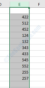
STEP 1- Select the column you want to filter by clicking on the column’s letter, upon successfully selecting the column excel will highlight the column as shown in following image.

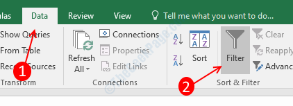
STEP 2- Click on the Data tab in the main menu and then click the filter button.

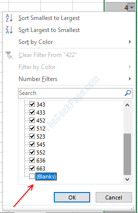
STEP 3- You will find an inverted triangle on right to the first number of your selected column, left-click on it. It will open up the filtering options pop-up. In the same pop up you can see all the numbers from your column are selected by default. Scroll down to the last until last number and uncheck blanks to disable the filtering of blank cells.

STEP 4- Apply the filters you want to apply on the column and then click Ok to save your settings.
Method 2 – Delete blank cells from the table
Blank cells hinder the filtering process in MS Excel so before you filter a column make sure that you don’t have any blank cells in between the data which would cause issues during the filtering data. To delete unwanted cells from the column you will have to delete the rows in which the blank cell is present.

To delete blank cell rows, left-click on the row number which has a blank cell, it will highlight the entire row. Right Click on the same row number and select the delete option. If you have multiple blank cells, first select all of them by holding Ctrl key and left-clicking on the row number and then delete all rows simultaneously.
NOTE: Double-check the row before deleting anything because if you delete anything important it will be hard to recover.
Method 3 – Ungroup Sheets
Filter options are disabled when you have grouped sheets in your document, all the options of the data tab would be greyed out if the document has grouped sheets. This is an annoying issue because you can’t figure out what’s wrong with the excel and why the data tab is disabled. As annoying, this problem is, the solution is very easy.

Select all the sheets by holding down Ctrl key and left-clicking on sheets, right-click on one of the sheets and select ungroup sheets option. You will find your Data tab is enabled now.
Method 4 – Remove Protection
Password protected spreadsheets are restricted to edit and therefore it can not be filtered. So, to filter data from the protected document first you have to remove the protection from the file. Follow these steps to unprotect your file. You will also need the password of the file
STEP 1- Go to the Review tab from the main menu of the Excel.
STEP 2- Click on the Unprotect Sheet, it will open a password pop-up.

STEP 3- Type in the password of the sheet and hit Enter. Your spreadsheet is now unlocked.

Method 5 – Unmerge Cells
If you have merged cells in your document, the filter option would not work so you have to unmerge the cells. Follow this process to unmerge the cells in your document.
STEP 1- Press Ctrl + F keys to open find and replace menu, Click on the options>> button to enlarge the popup.

STEP 2- Click on the Format button, it will open up another window.

STEP 3- Head over to the Alignment tab and select merge cells. Click Ok to save the settings.

STEP 4- Click on Find all button in the find and replace the window. It will list out the merged cells in the document.

STEP 5- Click on the inverted triangle button next to the merge and center button in the Home tab, select unmerge cells( without closing the find and replace window). It will automatically unmerge all the cells from the document.

Method 6 – Reapplying the Filter
In some cases due to some error filtering does not work out but re-applying the filter after clearing all the filters it works fine. Also, in many cases, it happens due to multiple filtering of the column so clearing the column of the filter helps.
STEP 1- Select the column by clicking the letter of the column

STEP 2- Click on the Clear Filter button in the Data tab (upper right of the filter button).

STEP 3 – Once again select the column and click on the filter button. Select your desired filter option and your data is filtered properly now.

This will solve your filtering issues in Microsoft Excel, comment down if you facing any problem following the procedure.