Let’s say you have a column of dates and another column of times in your Excel sheet. You need one extra column which has the combined values of both these columns. Well, under normal circumstances this could prove to be a headache. Even if you do manage to get the combining part right, the formatting part could be tricky. The format of dates and times could be all over the place and you might be facing great difficulties in fixing it. Well, fret no more, we are here to help, as always!
In this article, we explain through 2 different solutions how you can easily combine date and time values and populate a whole new column based on the combined values. Read on, to learn how!
Example Scenario
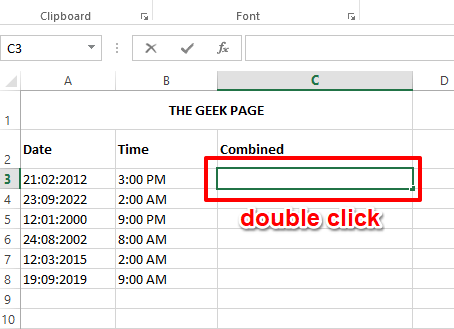
The example Excel sheet presented in this article has 3 columns namely Date, Time, and Combined. The Date column has date values, the Time column has time values and the Combined column is not yet populated. The requirement is to populate the column named Combined with the combined date and time values from their respective columns. Also to format the combined value appropriately using proper date and time formatting.
Solution 1: By Simply Adding the Date and Time Values Using Add Operation
Step 1: Double click on the first cell of the column that you want to populate using the combined date and time values.
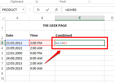
Step 2: Now, type in = <cell_id_of_date> + <cell_id_of_time>.
<cell_id_of_date> and <cell_id_of_time> have to be replaced with their respective cell ids as per your data arrangment.
In the example below, my initial date value is in cell A3, and my initial time value is in cell B3. Hence my formula would be =A3+B3.
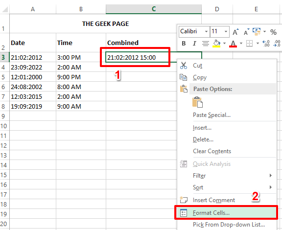
Step 3: If you hit the Enter key, you can see that your date and time values are now combined for the very first cell in the Combined column.
However, the format looks a bit odd and we need some fixing on that. For that, right click on the combined cell and click on the Format Cells option from the right click context menu.
Step 4: In the Format Cells window, click on the Number tab first.
Under the Category options, click on the Custom option next.
As next, type in the format that you want to apply to your combined data under the Type field. For example, I have given the format as dd/mm/yyyy hh:mm AM/PM. Under the sample field, you can see what a sample of your combined data would look like.
Once you are all set, hit the OK button.
Step 5: If you now look at your Excel sheet, your combined date and time value is now well-formatted.
To apply the formula throughout the column, click and drag down the small square shape present at the bottom right corner of your cell.
Step 6: There you are! You now have successfully applied the formatted formula to all the cells in the column. Enjoy!
Solution 2: By Using the Concatenate Formula
This method makes use of a formula function called concatenate. It takes in all the strings that need to be concatenated together and then returns the final concatenated string.
Step 1: Double click on the first cell of the column where you want the combined date and time value to come and then copy and paste the following formula onto it.
=CONCATENATE(TEXT(A3,"<date_format>")," ",TEXT(B3,"<time_format>"))
You need to replace <date_format> with the date format of your choice and <time_format> with the time format you require. If you want time to be displayed in AM/PM form, then you need to mention that at the end of the time format. An example formula with the date and time formats replaced is as below.
=CONCATENATE(TEXT(A3,"dd-mm-yyyy")," ",TEXT(B3,"hh:mm AM/PM"))
Step 2: If you hit the Enter key, you can see that you have the final date and time combined value in the cell where you applied the formula.
To apply the formula throughout the column, click and drag down the small square icon at the bottom right corner of the selected cell.
Step 3: Viola! Your formula is now applied throughout your column. Yes, it cannot get simpler than this, we agree too!
If you have any doubts following any of the steps, please drop us a comment, we would be happy to help. Do come back for more amazing articles on your favorite topics.


