When you have huge sets of data, analyzing the data often becomes more and more difficult. But really does it have to be so? Microsoft Excel provides an amazing inbuilt feature called Pivot table that can be used to easily analyze your huge data chunks. They can be used to efficiently summarize your data by creating your own custom reports. They can be used to calculate the sum of columns automatically, filters can be applied to them, the data in them can be sorted, etc. The operations you can perform on a pivot table and the ways how you can make use of a pivot table to ease your everyday excel hurdles are endless.
Read on, to learn how you can easily create a pivot table and to learn how you can efficiently organize it. Hope you enjoy reading the article.
Section 1: What is a Pivot Table
In the very basic terms, you can consider a pivot table as nothing but a dynamic report. There is a huge difference between reports and pivot tables though. Reports are static, they cannot provide any interaction. But unlike them, pivot tables let you view your data in many different ways. Also, a pivot table doesn’t require any formulae to form the data that it has. You can apply many filters on your pivot table and customize the data as per your requirement.
Section 2: Sample Data
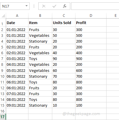
In this article, we have created a sample table with data for the pivot table creation. In the sample table, we created, there are columns for Date, Item, Units Sold, and Profit. We are mainly interested in finding the Total Profit for each day based on different items. Let’s see how this can be done with detailed steps and examples.
Section 3: How to Create a Pivot Table
Once you have the data ready, creating a pivot table is very easy.
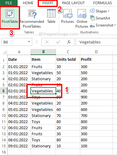
Step 1: Click anywhere inside your data. As next, click on the INSERT tab at the top ribbon. Now, click on the button named Pivot Table.
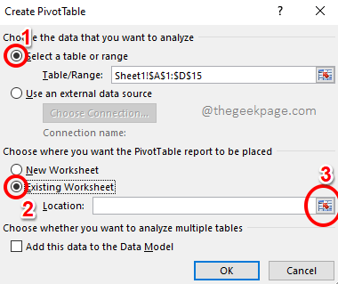
Step 2: Now the Create PivotTable window launches before you.
Under the Choose the data that you want to analyze section, by default the radio button corresponding to the option Select a table or range would be selected. If it’s not selected, please select it.
Now under the section Choose where you want the PivotTable report to be placed, you will have the option to create the pivot table in a New Worksheet or on the Existing Worksheet.
If you choose New Worksheet, the pivot table will be created in a different sheet. But since it’s easier to compare the pivot table with our sample data if they are both on the same sheet, I have chosen the option Existing Worksheet.
Once you have chosen the radio button corresponding to Existing Worksheet, click on the Select Cells button against the Location field.
Step 3: The Create PivotTable window would now be minimized. Click on the cell where you want your Pivot Table to start from. Once the cell is selected, click on the Select Cells button again to maximize the window.
Step 4: Hit the OK button once you are back at the Create PivotTable window.
Step 5: That’s it. Your PivotTable is now inserted into your Worksheet. In the sections below, let’s see how you can generate data in your pivot table and how you can manipulate the data.
Section 4: How to Generate Data in Pivot Table
Step 1: Let’s say you want to see the sum of profits. For that, you need not write any formula.
On the right window pane, where the PivotTable settings are present, you just need to click on the checkbox corresponding to the Profit column.
If you look at your Excel Worksheet, you can see that your PivotTable now has only one column and it reads Sum of Profit. It calculates the sum value of all the profits available in your sample data.
Step 2: Now let’s say you want to see the grand total of profit, but at the same time, you want to see the profit made for each day as well. In that case, check the checkbox corresponding to the Date column too, on the right window pane.
Now automatically, the Date column would come under the ROWS section of the pivot table and your pivot table would successfully display the profits made on each day. In the end, it shows the Grand Total of the profit made as well.
Step 3: Now, let’s try selecting the checkboxes corresponding to all the columns in your sample data. Well, that gives a perfect report in your pivot table, showing the profit made on each day by each item. Well, it cannot be more organized, we agree too!
Section 5: How to Apply Filters in Pivot Table
If you would like to view your pivot table only after applying some specific filters, there are ways to do that too. For example, if you want to view the profits made on each day by the item Fruits only, you can follow the steps below.
Step 1: Firstly, on the right side of the window, from the PivotTable Fields, drag and drop the Item field to the FILTERS section. This simply adds the filter Item to your pivot table.
Now on the pivot table, you will see the newly added filter Item. Click on the dropdown menu associated with it.
Step 2: Now click on the item Fruits and hit the OK button to filter the pivot table for Fruits only.
Note: You also have the option to apply multiple filters on your pivot table. You can do so by enabling the checkbox corresponding to Select Multiple Items marked in a circle in the screenshot below and then by choosing multiple fields.
Step 3: If you now look at the pivot table, you can see the Sum of Profit made on each day only by the item Fruits. Enjoy!
Section 6: How to Style a Pivot Table
Pivot tables are great and we all know that. But if a little bit of styling is also added, it can be greater. In this section, let’s see how you can add a preset styling to your pivot table to make it more readable and user-friendly.
Step 1: Firstly click somewhere on the pivot table.
Now, make sure you are at the HOME tab. As next, click on the dropdown Format as Table. From the list of styles available, choose any style of your choice.
Step 2: There you go! Your pivot table is now all set and ready to go. You can easily analyze the data using your brand-new pivot table without the help of any formulae!
Please tell us in the comments section if you have any questions regarding any of the steps, we are always happy to help, and just a comment away.
Stay tuned for more amazing technical articles!


