Excel doesn’t provide an inbuilt formula to return the name of the active Excel worksheet right away. However, there could be situations where you need to dynamically populate the value of your active sheet in your Excel file. For example, if the name of the table on your sheet has to be the name of the sheet itself and if you hardcode the table name, and if you change the sheet name later, the table name also has to be changed manually. But if the name of the table is dynamically populated, say using a formula, then if the sheet name changes, the name of the table also changes automatically.
As mentioned already, though the requirements are very much a possibility, there is no straight-cut formula using which you can extract the name of the active sheet. However, we do have some formula combinations using which you can successfully extract the name of the active sheet. Read on, to learn how!
Section 1: How to Get the Name of the Current Sheet Using the Combination of Right, Cell, Find, and Len Functions
Section 1.1: Complete Formula
The first step would be to make sure that you have saved your Excel sheet. If you haven’t saved your Excel document, save it first, else this formula wouldn’t work.
To save the document, you can simply press the CTRL + S keys together, navigate to the location where you want to save your document, give a name to the file and then finally save it.
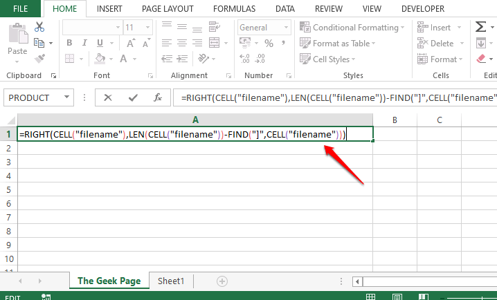
Step 1: Once you have saved the Excel document, simply double click on any cell. Once you enter the edit mode, copy and paste the following formula and hit the Enter key.
=RIGHT(CELL("filename"),LEN(CELL("filename"))-FIND("]",CELL("filename")))
Note: Don’t worry seeing the length of the formula, in the section below, we have explained the formula in detail.
Step 2: Once you hit the Enter key, you can see that the name of the current sheet, in the example below the sheet name is The Geek Page, is successfully returned on the cell where the formula was entered. Yes, it’s simple, we agree too. But if you would like to know how the formula worked, you can refer to the section below.
Section 1.2: Formula Explanation
In this section, let’s take the lengthy formula from the section above, split it and figure out what really is happening and how it is returning the name of the current sheet successfully.
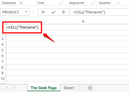
Step 1: The very first part of the formula is =CELL(“filename”). The cell function takes only one argument. It returns the complete address of the cell, including the file location of the sheet and the current worksheet name.
Step 2: If you look at the screenshot below, if you hit the Enter key, you get the whole filename including the current sheet name at the end.
Step 3: As you can see, the sheet name is at the very end of the filename. To be precise, whatever comes after the right square brace, ], is the sheet name. So, let’s use the FIND function to find the index value of the square brace character. After we find that index, let’s find which all characters come after it, which is essentially the sheet name.
The FIND function takes in 2 arguments, one is the character whose index is to be found, and the second is the string where the search is to be performed. So our FIND function would look like the following in this particular case.
=FIND("]",A1)
A1 is the cell id of the cell that contains the filename that we found using the CELL function. If your filename is in a different cell, you should give that cell id instead of A1.
Step 4: The FIND function returned the value 65. This means that the right square brace is at the 65th position. So we need to extract everything from the filename that comes after the 65th position, i.e., everything that comes after the right square brace.
Step 5: To extract everything that comes after the 65th position, we first need to know how many characters are to be extracted after the 65th position. To make it more simple, we need to know how many characters precisely our current sheet name has. For that, let’s use the LEN function. The function is as follows.
=LEN(A1)-FIND("]",A1)
The above formula simply returns the length of the sheet name. It is found out by calculating the length of the filename first, using LEN(A1), and then subtracting the length of the filename till the right square brace, which is 65.
Step 6: The above formula returns 13, which is the length of the current sheet name, The Geek Page.
Step 7: So we now have the source string, which is the complete filename and we know that the current sheet name is of 13 characters and that it is at the end of the filename. So, if we extract 13 characters from the very right of the filename, we get the current sheet name.
Now, let’s extract the sheet name using the RIGHT function straight away. The RIGHT function is as follows.
=RIGHT(A1, LEN(A1)-FIND("]",A1))
The RIGHT function takes in 2 arguments, one is the string from which the substring is to be extracted, and the second is the number of characters that need to be extracted from the right part of the parent string.
Now, the following screenshot tells you this in detail. The RIGHT function takes in the filename and the length of the current sheet. So from the filename, RIGHT string will extract the sheet name, which is of 13 characters as calculated from the steps above, from the very right side of the string.
Step 8: There you go! The name of the active sheet is now successfully extracted!
Step 9: The name is extracted successfully, but there is one small dependency. Our formula has a dependency on the cell where the CELL function is defined. We keep referring to A1. One thing is, we might not want the full filename in our document, so it could be a huge inconvenience to have it on the document. Another thing is that if we delete it, our formula will no longer work as it has a dependency. So let’s remove the dependency.
For that, double click on the cell where the CELL function is defined and copy the entire formula. You can copy the formula by selecting it and then by pressing the keys CTRL + C together.
Step 10: Now in our RIGHT formula, replace A1 with the CELL function that you copied in Step 9. There are 3 occurrences of A1 in the RIGHT formula, so all 3 have to be replaced.
Step 11: The below screenshot shows what the RIGHT formula should look like after the replacements are made.
Step 12: If you hit the Enter key or click elsewhere, you can see that the current sheet name is successfully extracted. Also, since there is no dependency anymore, you can delete the A1 cell. Enjoy!
Section 2: How to Get the Name of the Current Sheet Using the Combination of Mid, Cell, and Find Functions
This is another formula combination using which you can find the name of the active sheet. In this formula, instead of using the RIGHT function, we use the MID function. The formula is as follows.
=MID(CELL("filename"),FIND("]",CELL("filename"))+1,255)
In the Excel document, double click on any cell and simply copy-paste the above formula and hit the Enter key. You would get the name of the active sheet returned on the cell you entered the formula at.
Note: The MID function returns the substring from the main string if we give the starting position of the substring and its length.
Please also note that even for this formula to work, you should first have the document saved somewhere, else you will get the Value error.
Even though there is no straightforward formula in Excel using which you can straight away get the name of the active sheet, using either of the above formula combinations, you can get your desired result.
Please tell us in the comments section if you have any concerns regarding any of the steps.
Stay tuned!


