There are so many ways to find and eliminate duplicate data entries from your Excel file. But all these ways mostly work after you have entered all the data. But have you been wondering whether you can get Excel to warn you as and when you type in a duplicate value? Have you been wondering whether you can somehow get Excel to prevent you from entering a duplicate value, say, maybe with the help of an Error window? Well, we have perfectly read your mind!
In this article, we tell you in detail how you can apply a duplicate data entry prevention rule on a range of cells that you select. We also tell you how you can customize the error message window that pops up when you enter a duplicate value. And if you are confused about whether the rule can ever be reverted, we have a solution for that as well. So what are you waiting for, let’s dive straight into the article, shall we?
Also Read: How to Remove or Highlight Duplicates in Excel
Section 1: How to Prevent Duplicate Value Entries
Step 1: Firstly, select the range of cells where you don’t want to allow duplicate data entries.
Once the range of cells is selected, click on the DATA tab from the top ribbon.
Now click on the dropdown button named Data Validation and click on the Data Validation option from the list of options available.
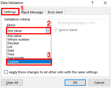
Step 2: On the Data Validation window, click on the Settings tab at the top.
Now, click on the dropdown button associated with the option Allow.
From the list of options available, click on the one that says Custom.
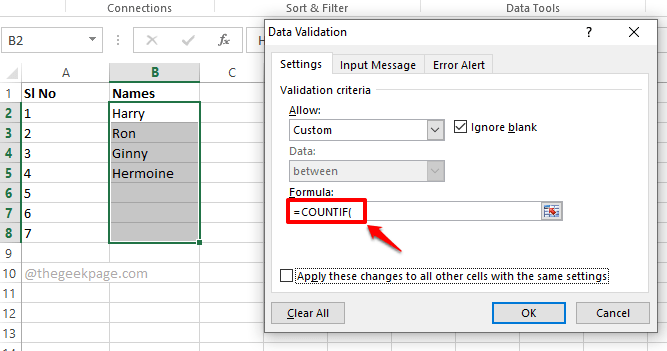
Step 3: Under the Formula field, type in or copy and paste the following next.
=COUNTIF(
Step 4: After that, in the background, select the range of cells where you want to apply the duplicate prevention rule.
Now, if you look at your Data Validation window, you can see that the portion after =COUNTIF( is filled partially. Let’s go ahead and complete the formula in the coming steps.
Step 5: The next step would be to simply press the F4 key. This would add $ signs in your formula, locking those values where $ got added.
Step 6: As next, put a comma, and then on the Excel sheet, click on the first cell in your selected range of cells.
Step 7: To complete your formula, now you just need to type in or copy and paste the following under the Formula field.
)=1
Your final formula should look like the one in the following screenshot. Obviously, the cell ids will be different.
Once you are all done, hit the OK button.
Step 8: That’s it. If you now try to type in a duplicate value, to a cell where your duplicate prevention validation rule is applied, you will get the following error window, that doesn’t let you proceed until your enter a unique value in your cell.
Section 2: How to Customize the Duplicate Entry Error Message
If you do not want the default error message window to be shown while a duplicate entry is detected, then you can create your own custom error message window following the steps below.
Step 1: Once again, select the range of cells where you have applied the rule in the section above.
Then click on the DATA tab from the top ribbon.
Now click on the Data Validation dropdown button and then click on the Data Validation option from the list of options available.
Step 2: On the Data Validation window, click on the Error Alert tab at the right end.
Now, under the Style dropdown menu, choose the style Stop. This will prevent a duplicate value from being entered.
Note: The other styles available in the Style dropdown menu are Warning and Information. Only the style named Stop would prevent duplicate values from being entered. The other 2 styles would let you continue your data entry after showing a warning or information message respectively.
Once the style is selected, under the Title field, you can type in a title for your error window. I have typed in my title as Duplicate Entry Found.
You also have the option to set the error message that you want to be shown whenever a duplicate value is entered. You can type in the error message for your error window under the Error message field. The message I have entered is Hey there! That’s a duplicate entry that you are trying to enter!.
Hit the OK button once you are all done.
Step 3: That’s it. If you now try to enter a duplicate value, you can see your custom error message window popping up, replacing the default one. Enjoy!
Section 3: How to Remove the Data Validation Rule
If in the future you would like to allow duplicate values on the range of cells where you set the duplicate prevention rule, you can do so easily by following the steps below.
Step 1: Select the range of cells where the duplicate prevention rule is applied. As next, click on the DATA tab from the top ribbon.
Now click on the Data Validation dropdown button and then select the Data Validation option.
Step 2: On the Data Validation window, under the Settings tab, choose the dropdown option Any value from the Allow dropdown menu.
Hit the OK button to proceed. That’s it. You can now enter as many duplicate values as you want.
Please tell us in the comments section if you have any concerns regarding any of the steps.
Stay tuned for more amazing tricks, tips, how-tos, and hacks.


